Planned research · not yet implemented

FUTURE PROJECT C · NAVIGATION & STATE ESTIMATION

Autonomous Navigation & Multi-Sensor Fusion

A real-time navigation estimator fusing GPS/GNSS, IMU and wheel odometry — built to stay stable when satellite positioning degrades.

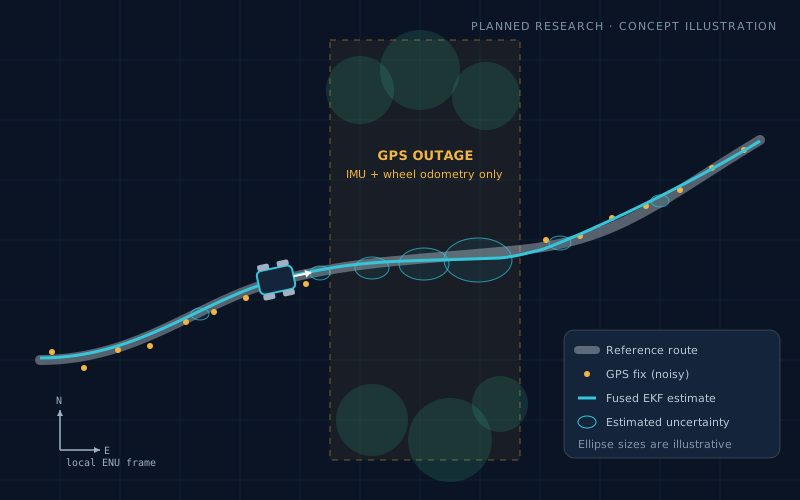
The plan is to design and implement a navigation system that estimates a vehicle's or robot's position, velocity and heading by combining complementary sensors, and keeps producing a trustworthy estimate — with an honest uncertainty — during temporary GPS outages.

It extends my low-cost GPS navigation and fleet-tracking platform and my Kalman-filtering work. The goal is a complete, testable engineering system — real hardware, a modular ROS 2 architecture and measured results — not only a fusion algorithm.

Explore the Architecture How It Will Be Tested All Future Projects

Concept illustration: a ground robot follows a route with noisy GPS fixes around it and a smooth fused estimate. In a shaded GPS-outage zone under trees, uncertainty ellipses grow while the robot relies on IMU and odometry, then shrink when GPS returns. — Concept illustration Fused estimate through a GPS outage; uncertainty grows on dead reckoning and contracts when fixes return. Illustrative, not measured.

Status: Planned R&D; estimator, robot integration and tests are not yet built
Builds on: GPS tracking platform (Raspberry Pi 4), Kalman & adaptive filtering
First milestone: Live GPS/IMU estimator on a Pi 4, compared quantitatively with GPS-only
Demonstrator: Small ground robot: GPS + IMU + wheel encoders, LiDAR later

Problem & motivation

Why One Sensor Is Not Enough

GPS gives absolute position but is noisy, updates slowly and can disappear under trees, near buildings or in tunnels. An IMU measures motion at a high rate but drifts without bound. Wheel encoders measure how far the wheels turned — not how far the robot moved when they slip.

Each sensor's weakness is another's strength, and a Kalman-filter-based estimator can combine them according to their uncertainty. But connecting several sensors does not automatically improve navigation: each one must be calibrated, time-aligned, modelled and validated, and the fused result must be shown to beat the simpler alternatives under measured conditions.

Planned engineering objectives

Estimate position, velocity and heading in real time.
Fuse GPS and IMU with a Kalman-filter-based estimator.
Detect GPS outages, noisy measurements and inconsistent sensor data.
Evaluate fusion against GPS-only and IMU-only solutions.
Keep the design modular for wheel encoders, magnetometers, LiDAR or visual odometry.
Demonstrate results on recorded datasets and real-world tests.

Complementary sensor characteristics

Qualitative characteristics; actual performance depends on the specific devices and will be measured.
Sensor	Measures	Strength	Weakness
GPS / GNSS	Absolute position, time, possibly velocity	No long-term drift	Noise, low rate, multipath and outages; heading unreliable when stationary
IMU (6- or 9-axis)	Acceleration, angular rate (and magnetic field)	High rate, independent of the environment	Bias and noise integrate into growing drift; magnetometer is disturbed by nearby metal
Wheel encoders	Wheel rotation	Good short-term distance and turn rate	Wheel slip, scale-factor errors, no absolute position
2-D LiDAR (later)	Ranges to the surroundings	Obstacles; localisation against a map	Needs geometric features; cost and processing load
Camera (later)	Images	Visual odometry, rich context	Lighting, texture and calibration dependence

Proposed architecture

From Sensors to a Navigation Output with Uncertainty

Each sensor driver and estimator is a separate module that can be tested on its own, and a low-cost sensor can later be replaced by a better one without redesigning the system.

Navigation system architecture

Proposed design

Sensor inputs
- GPS / GNSS
- IMU
- Wheel encoders
- Optional LiDAR / camera
Data acquisition & synchronisation
- Drivers
- Timestamps
- Coordinate transforms
- Calibration
- Sensor health
State estimation & sensor fusion
- IMU motion propagation
- GPS corrections
- Kalman filtering
- Outlier rejection
Navigation output
- Position
- Velocity
- Heading
- Uncertainty
Monitoring, analysis & control interface

Monitoring & analysis
Live map, trajectory, sensor status, error reports.
Navigation & control
Waypoint following, obstacle response, safe-stop behaviour.

How the system would work

IMU propagation
Angular rates and accelerations at high frequency propagate the state between corrections.
Odometry aiding
Wheel-encoder speed and turn rate constrain motion when available.
GPS correction
Absolute position (and possibly velocity) corrects accumulated drift, weighted by its uncertainty.
Publish state + health
Estimated state, covariance and sensor-health indicators for the navigation layer.

LiDAR and camera data would not be pushed into the same filter at first. They would provide separate localisation estimates or obstacle information, integrated later through a well-defined interface.

Concept diagram Frame tree following the ROS map → odom → base_link convention, managed with TF2.

Coordinate frames & transforms

Define the global frame, local navigation frame, robot body frame and every sensor frame explicitly, and manage them with ROS 2 TF2. Geographic coordinates are converted carefully to the local frame, and three different "headings" are kept apart:

True heading — the direction the robot body points, relative to true north.
Magnetic heading — the same, from a magnetometer, affected by declination and local interference.
Course over ground — the direction of travel from GPS velocity, undefined when stationary.

Heading is not free. A stationary single-antenna GPS cannot give heading. A magnetometer helps but is easily disturbed; dual-antenna GNSS, motion-based estimation or a well-calibrated inertial system may be needed, depending on the accuracy required.

Sensor-fusion algorithm design

Four Fusion Stages, Each Judged Against the Last

This is where Kalman-filter and tracking experience becomes the central advantage. Each stage must show a measured improvement over the previous one — including where it does not help.

GPS baseline
Record raw GPS; compute position and velocity, fix quality and satellite data, stationary scatter and error against a trusted reference.
sets the bar to beat
GPS + IMU
An EKF (or an existing ROS 2 estimator): the IMU propagates the state, GPS corrects the drift; uncertainty tracked in the covariance.
core estimator
+ Wheel odometry
Adds motion information when GPS is unreliable — while recognising that slip causes drift and encoders give no absolute position.
robot_localization (EKF/UKF)
LiDAR or visual localisation
Only after stages 1–3 are stable: LiDAR mapping/localisation, or visual(-inertial) odometry, for areas with poor satellite positioning.
environment-dependent

Off-the-shelf firstStart with the ROS 2 robot_localization package, which supports EKF and UKF estimation and fuses IMU, odometry and GPS-derived position. It gives a tested baseline quickly.

Own estimator next (research)Implement a custom EKF and an adaptive measurement/process-noise strategy, compared fairly against the fixed-noise baseline on identical recorded data.

Ultrasonic sensors are not LiDAR. They are useful for cheap short-range obstacle detection, but provide little information for precise global positioning.

Mathematical foundations

Inertial Propagation, GPS Correction and Dead Reckoning

A simplified strapdown-inertial formulation in a local frame. Worked numbers are arithmetic illustrations, not sensor specifications.

Navigation state

Position, velocity, attitude and sensor biases

x = {[\begin{matrix} p & v & q & b_{a} & b_{g} \end{matrix}]}^{T}

$p$: Position in the local navigation frame (3).
$v$: Velocity (3).
$q$: Orientation as a unit quaternion (4), avoiding Euler-angle singularities.
$b_{a}, b_{g}$: Accelerometer and gyroscope biases (3 + 3), estimated online because they change with temperature and time.

In an error-state EKF the attitude error is three-dimensional, giving a 15-element error state.

IMU mechanisation

Continuous-time propagation

\dot{p} = v

\dot{v} = R (q) (\tilde{a} - b_{a}) + g

\dot{q} = \frac{1}{2} q \otimes [\begin{matrix} 0 \\ \tilde{ω} - b_{g} \end{matrix}]

{\dot{b}}_{a} = n_{b a}, {\dot{b}}_{g} = n_{b g}

$\tilde{a}, \tilde{ω}$: Measured specific force and angular rate in the body frame.
$R (q)$: Rotation from body to navigation frame.
$g$: Gravity vector in the navigation frame.
$n_{b *}$: Small white-noise inputs: biases modelled as slow random walks.

Discretised and linearised, this gives the EKF prediction $P_{k | k - 1} = F_{k} P_{k - 1} F_{k}^{T} + Q_{k}$ .

GPS correction & outlier rejection

Measurement model with lever arm and gate

z_{GPS} = p + R (q) l + η_{GPS}

ν_{k}^{T} S_{k}^{- 1} ν_{k} \leq χ_{3, 0.99}^{2}

$l$: Lever arm: offset from the IMU to the GPS antenna, measured on the robot.
$η_{GPS}$: GPS noise, covariance set from measured stationary scatter and reported fix quality — not arbitrary guesses.
$χ^{2}$: Chi-square gate (≈ 11.34 for 3 DoF at 99 %): implausible jumps are rejected and logged rather than fused.

Dead reckoning

Differential-drive wheel odometry

v = \frac{r (ω_{R} + ω_{L})}{2}

ω = \frac{r (ω_{R} - ω_{L})}{b}

x_{k + 1} = x_{k} + v Δ t \cos θ_{k}

y_{k + 1} = y_{k} + v Δ t \sin θ_{k}

θ_{k + 1} = θ_{k} + ω Δ t

$ω_{R}, ω_{L}$: Right and left wheel angular speeds from the encoders.
$r, b$: Wheel radius and wheel separation — both calibrated, because small errors bias every step.
$θ$: Heading; odometry heading error accumulates and bends the whole path.

Why outages are time-limited

Drift from an uncorrected bias

δ p (t) \approx \frac{1}{2} δ b_{a} t^{2}

δ ψ (t) \approx δ b_{g} t

A residual accelerometer bias $δ b_{a}$ grows into position error quadratically; a residual gyro bias grows heading error linearly, which then bends the dead-reckoned path.

Arithmetic example: $δ b_{a} = 0.05$ m/s² gives ≈ 2.5 m after 10 s but ≈ 22.5 m after 30 s. That is why dead reckoning continues only while its covariance stays acceptable, after which the system signals degraded navigation and enters a safe behaviour.

Evaluation

Accuracy and consistency

RMSE = \sqrt{\frac{1}{N} \sum_{k = 1}^{N} {‖ {\hat{p}}_{k} - p_{k}^{ref} ‖}^{2}}

ϵ_{k} = e_{k}^{T} P_{k}^{- 1} e_{k}

RMSE says how wrong the estimate is; the normalised estimation error squared $ϵ_{k}$ says whether the filter knows how wrong it is. A smooth trajectory alone does not prove accuracy — the reported uncertainty must be consistent with the observed errors.

Proposed hardware · ground-robot demonstrator

Minimum Useful Configuration First

A small ground robot is safer and easier to test repeatedly than a car, and the same principles carry over to vehicles and drones. Hardware is expanded only after the first estimator has been evaluated.

01 · Onboard computer
Raspberry Pi 4 Model B, 8 GB
Ubuntu 24.04, ROS 2 Jazzy, drivers, estimation, logging and visualisation interfaces.
Platform exists (Project 03)
02 · GPS / GNSS
ATGM336H-5N or better
Position, time and possibly velocity. Its accuracy is assessed before it is ever used as a reference.
Receiver exists (Project 03)
03 · IMU
Calibrated 6- or 9-axis IMU
Acceleration and angular rate (plus magnetometer on 9-axis). Chosen for bias stability, vibration sensitivity, rate and driver support.
To acquire
04 · Wheel encoders
Recommended for a ground robot
Dead reckoning between GPS updates. Calibrate wheel diameter, counts and separation; expect slip errors.
If not already fitted
05 · Optional LiDAR
2-D scanning LiDAR
Added after GPS/IMU/encoder fusion is validated: obstacle detection and, with mapping software, localisation.
Later investment

Practical sequencing: with the existing GPS and UGV available, the first purchase is only the IMU. My existing Raspberry Pi 4 six-wheel-motor UGV could serve as the base if its chassis, motor drivers, encoders and power supply prove suitable — no second robot needs to be built from scratch.

Demonstrator phases

Phase A — GPS/IMU navigation
Raspberry Pi, GPS receiver and IMU; log raw and fused data and compare errors against a reference trajectory.
Phase B — dead reckoning & obstacles
Wheel encoders for motion estimation; 2-D LiDAR for mapping and obstacles; ultrasonic sensors for cheap short-range detection.
Phase C — autonomous navigation
Map-based localisation, route planning and waypoint following; stop or re-plan when an obstacle appears.

Embedded Linux & ROS 2 implementation

Tested Middleware, Own Estimation and Evaluation

Rather than writing every subsystem from scratch, the plan builds custom estimation and evaluation modules around tested ROS 2 middleware and drivers.

Proposed software; documentation sources: ROS 2 Jazzy, robot_localization and Nav2.
Component	Proposed technology	Purpose
Operating system	Ubuntu 24.04 LTS	Onboard computer
Robotics middleware	ROS 2 Jazzy	Sensor communication and integration
Programming	Python first; C++ where performance-critical	Estimation, drivers, real-time processing
State estimation	robot_localization, then own EKF	GPS/IMU/odometry fusion
GNSS integration	nmea_navsat_driver or receiver-specific driver	GPS message acquisition
Visualisation	RViz2	Position, trajectory, frames, sensor data
Data analysis	NumPy, pandas, Matplotlib	Offline experiments and evaluation
Mapping & autonomy	Nav2, occupancy grids, localisation package	Waypoints, obstacle-aware planning
Datasets & playback	ROS 2 bags, CSV exports	Repeatable experiments and debugging

Proposed project structure

autonomous_navigation/
├── src/
│   ├── gps_driver/
│   ├── imu_driver/
│   ├── wheel_odometry/
│   ├── coordinate_transforms/
│   ├── sensor_calibration/
│   ├── state_estimator/
│   ├── sensor_health_monitor/
│   ├── localization_evaluator/
│   ├── waypoint_navigation/
│   └── dashboard/
├── config/
│   ├── sensors.yaml
│   ├── ekf.yaml
│   └── robot.yaml
├── launch/
├── datasets/
├── results/
├── tests/
└── README.md

The custom estimator must be testable against the ROS 2 estimator using identical recorded sensor data.

Engineering challenges & limitations

What Separates a Credible System from a Demo

Timing
Time synchronisation
GPS and IMU arrive at different rates and latencies.
Approach: preserve timestamps, measure offsets, never treat a delayed measurement as current; account for ROS 2 message timing.
Calibration
Sensor uncertainty
Biases, mounting orientation, GPS noise and encoder scale factors all matter.
Approach: configure covariances from measurements, not guesses.
Outages
Degraded GPS
Implausible jumps, poor fixes, stale data and sensor disagreement.
Approach: detect and gate; propagate on inertial/odometry only while uncertainty is acceptable, then signal degraded mode and stop safely.
Slip
Wheel slip & turning
Rapid turns and low-traction surfaces corrupt odometry.
Approach: cross-check odometry against IMU yaw rate; compare baseline and adaptive estimators.
Reference
Ground truth
Ordinary GPS cannot measure its own accuracy.
Approach: survey-grade/RTK GNSS reference, a known reference trajectory or validated ground-truth points.
Compute
Embedded budget
A Raspberry Pi has limited CPU for estimation plus logging and visualisation.
Approach: measure latency, CPU and memory; move hot paths to C++.

Testing & performance metrics

Proving That Fusion Works

A test framework is built before full autonomy. A successful result shows measurable improvement — and also the conditions where fusion does not improve the result.

Test 1 — stationary stability
GPS-only vs. fused positions while stationary: scatter, drift and false motion, against an RTK-class reference.
Test 2 — normal movement
A repeatable path with straights, turns, stops and speed changes; trajectory error and heading response.
Test 3 — degraded GPS
Replay with simulated gaps and noise, then controlled real tests under trees or near buildings; drift and recovery time.

Plus Test 4 — rapid turns and different traction, comparing the baseline EKF with the proposed adaptive estimator.
Metric	What it tells us
Horizontal position RMSE	Overall position-estimation error
95th-percentile position error	Performance during larger deviations
Velocity RMSE	Quality of motion estimation
Heading error	Orientation or course accuracy against a valid reference
Drift during GPS outages	How quickly dead reckoning becomes unreliable
Recovery time	Time to return to acceptable error after GPS resumes
Processing latency	Time from measurement arrival to published estimate
CPU and memory usage	Suitability for embedded deployment
Availability	Share of time the estimate meets defined quality requirements
Filter consistency (NEES)	Whether reported uncertainty matches observed error

Phased development

Six Stages over About Six Months, Part-Time

Planning estimates, not guaranteed dates. If the existing robot already has working ROS 2 communication and usable encoders, the early stages may be shorter.

01Weeks 1–3
Sensor acquisition & baseline
- Read GPS and IMU with timestamps
- ROS 2 topics
- Repeatable datasets
Deliverable: a sensor-logging and visualisation demonstration.
02Weeks 4–6
GPS/IMU estimator
- Validated EKF baseline
- Coordinate transforms
- Sensor calibration
Deliverable: fused position and motion on a live map.
03Weeks 7–10
Dead reckoning & evaluation
- Add wheel odometry
- Log GPS outages
- GPS-only vs. odometry-only vs. fused
Deliverable: reproducible test reports.
04Weeks 11–14
Custom & adaptive estimator
- Own EKF implementation
- Adaptive noise strategy
- Comparison on identical datasets
Deliverable: fixed vs. adaptive comparison report.
05Weeks 15–19
Environmental sensing
- LiDAR obstacle detection
- Mapping / localisation if appropriate
Deliverable: a robot that estimates its state while detecting nearby obstacles.
06Weeks 20–24
Waypoint navigation & release
- Nav2 or similar stack
- Safe stopping
- Repeatable trials
Deliverable: architecture, demonstration video and performance results published.

First milestone: a live GPS/IMU navigation estimator running on the Raspberry Pi 4, with recorded sensor data and a quantitative comparison between GPS-only and fused estimates — before any LiDAR or autonomous control.

Expected contribution

Expected Contribution & Research Direction

The distinctive contribution is not the use of a Kalman filter by itself, but the engineering of a complete, testable navigation solution: uncertainty management, sensor integration, real-world validation and, potentially, an adaptive estimator.

Existing expertise applied
GPS tracking, Kalman filtering, target-motion estimation, sensor-data integration, coordinate transformations, real-time software, Linux and system testing.
New competencies to demonstrate
Inertial navigation, IMU calibration, odometry, ROS 2 integration, robotics coordinate frames, LiDAR localisation and autonomous waypoint navigation.

Proposed project lead

Mohammed Ismail Ali Attala

Senior Systems Engineer · C4I/C2 Integration · Tracking & Navigation

Open to collaboration on GPS-degraded localisation, mobile robotics and navigation research.

Potential applications

Autonomous ground robots and civilian vehicle navigation
GPS-degraded localisation
Fleet and asset tracking
Drone navigation research

Contact & Collaboration

Working on Robots, Vehicles or Drones?

I welcome discussions about multi-sensor navigation, state estimation, GPS-degraded positioning and ROS 2 integration.

Send an Email LinkedIn Back to Future Projects

Autonomous Navigation & Multi-Sensor Fusion

Why One Sensor Is Not Enough

Planned engineering objectives

Complementary sensor characteristics

From Sensors to a Navigation Output with Uncertainty

Navigation system architecture

Sensor inputs

Data acquisition & synchronisation

State estimation & sensor fusion

Navigation output

Monitoring, analysis & control interface

Monitoring & analysis

Navigation & control

How the system would work

IMU propagation

Odometry aiding

GPS correction

Publish state + health

Coordinate frames & transforms

Four Fusion Stages, Each Judged Against the Last

GPS baseline

GPS + IMU

+ Wheel odometry

LiDAR or visual localisation

Inertial Propagation, GPS Correction and Dead Reckoning

Position, velocity, attitude and sensor biases

Continuous-time propagation

Measurement model with lever arm and gate

Differential-drive wheel odometry

Drift from an uncorrected bias

Accuracy and consistency

Minimum Useful Configuration First

Raspberry Pi 4 Model B, 8 GB

ATGM336H-5N or better

Calibrated 6- or 9-axis IMU

Recommended for a ground robot

2-D scanning LiDAR

Demonstrator phases

Phase A — GPS/IMU navigation

Phase B — dead reckoning & obstacles

Phase C — autonomous navigation

Tested Middleware, Own Estimation and Evaluation

Proposed project structure

What Separates a Credible System from a Demo

Time synchronisation

Sensor uncertainty

Degraded GPS

Wheel slip & turning

Ground truth

Embedded budget

Proving That Fusion Works

Test 1 — stationary stability

Test 2 — normal movement

Test 3 — degraded GPS

Six Stages over About Six Months, Part-Time

Sensor acquisition & baseline

GPS/IMU estimator

Dead reckoning & evaluation

Custom & adaptive estimator

Environmental sensing

Waypoint navigation & release

Expected Contribution & Research Direction

Existing expertise applied

New competencies to demonstrate

Mohammed Ismail Ali Attala

Potential applications

Working on Robots, Vehicles or Drones?