PROJECT 04 · ADVANCED TRACKING ALGORITHMS

Adaptive Kalman Filtering for Maneuvering Targets

Adaptive State Estimation Under Abrupt Motion Changes

A Kalman filter tracks well while a target moves the way its model expects. When an aircraft or drone turns, accelerates or breaks away abruptly, the prediction falls behind and the error grows.

This project develops an adaptive Kalman tracking algorithm that detects the maneuver, shifts the predicted track position towards the target's new motion and recenters the validation gate there. The aim is to keep the track through the maneuver without the computational load of running several motion models in parallel, as the Interacting Multiple Model (IMM) algorithm does.

Explore the Algorithm Simulation Results

Back to all projects

Simulation plot in X and Y coordinates in kilometres: a target trajectory with straight segments and several sharp turns. Measurements are shown in red, the standard Kalman filter in black, IMM in green and the adaptive Kalman filter in blue. Two zoomed insets show turn regions where the standard Kalman filter estimate swings wide of the measurements while the adaptive and IMM estimates stay closer. — Simulation result Simulated maneuvering target: measurements, standard KF, IMM and the adaptive Kalman filter (scenario 1).

Baseline: Linear discrete-time Kalman filter
Key idea: Shift the predicted position and recenter the gate after maneuver detection
Compared with: Standard Kalman filter and IMM, in simulation
Evidence: Two simulated scenarios, compared visually as trajectory plots

The engineering problem

Rapid Evasive Maneuvers

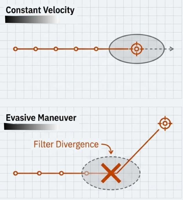
A standard Kalman filter predicts the next position with a fixed motion model. A constant-velocity model assumes the target keeps its heading and speed between scans, treating any small change as process noise. For a target that really flies straight, that assumption produces accurate, smooth estimates.

Aircraft and drones do not always fly straight. During a maneuver the target can change heading, accelerate, decelerate or reverse direction within a few scans. The filter keeps predicting along the old path, so the gap between prediction and measurement, the residual, grows. Every update then corrects only part of that gap, the estimate lags behind the target and, in severe cases, the track can lose its measurements altogether and diverge.

Two panels. Top, constant velocity: past positions lie on a straight line and the next position falls inside the prediction ellipse. Bottom, evasive maneuver: the target turns sharply away, the prediction ellipse stays on the old straight path and is marked as filter divergence. — Project illustration Top: the prediction gate keeps up with constant-velocity motion. Bottom: after an abrupt turn the target leaves the gate and the filter can diverge.

Constant-velocity assumption
Heading and speed are treated as constant; deviations are absorbed by process noise.
Abrupt heading change
The target turns, but the prediction continues along the previous course.
Sudden acceleration or deceleration
Speed changes faster than the model allows, so predicted positions over- or under-shoot.
Unexpected direction change
An evasive break or reversal moves the target far from its predicted position.
Model mismatch → growing residuals
Measurements no longer agree with predictions, and estimation errors build up scan after scan.
Possible divergence
Under severe maneuvers the track can fail to associate its own measurements and be lost.

Central question

How can a tracking filter adapt rapidly to a maneuvering target without unnecessarily increasing computational complexity?

Baseline algorithm

Standard Kalman Filter Fundamentals

The discrete-time linear Kalman filter alternates between predicting the target's state and correcting it with each new measurement. A simple two-dimensional state holds position and velocity:

x_{k} = {[p_{x}, p_{y}, v_{x}, v_{y}]}^{T}

PREDICT Project the state ahead

State prediction

${\hat{x}}_{k | k - 1} = F_{k} {\hat{x}}_{k - 1 | k - 1}$

Projects the previous estimate one scan ahead with the assumed motion model.
Covariance prediction

$P_{k | k - 1} = F_{k} P_{k - 1 | k - 1} F_{k}^{T} + Q_{k}$

Propagates the uncertainty and adds process noise, so the prediction is less certain than the last estimate.

What the gain does. A large gain trusts the measurement; a small gain trusts the prediction. The estimates are only as good as the motion model and the noise settings behind that balance.

UPDATE Correct with the measurement

Measurement residual

$r_{k} = z_{k} - H_{k} {\hat{x}}_{k | k - 1}$

The innovation: how far the measurement lies from where the filter expected it.
Residual covariance

$S_{k} = H_{k} P_{k | k - 1} H_{k}^{T} + R_{k}$

How large the innovation is expected to be, combining prediction and sensor uncertainty.
Kalman gain

$K_{k} = P_{k | k - 1} H_{k}^{T} S_{k}^{- 1}$

Balances trust between the prediction and the measurement.
State update

${\hat{x}}_{k | k} = {\hat{x}}_{k | k - 1} + K_{k} r_{k}$

Corrects the prediction by the gain-weighted residual.
Covariance update

$P_{k | k} = (I - K_{k} H_{k}) P_{k | k - 1}$

Reduces the uncertainty after the measurement has been used.

Notation

$\hat{x}$: Estimated target state (e.g. position and velocity).
$F_{k}$: State-transition matrix: the assumed motion model.
$P$: State-estimation error covariance: how uncertain the estimate is.
$Q_{k}$: Process-noise covariance: how much the motion may deviate from the model.
$z_{k}$: Measurement vector received at scan k.
$H_{k}$: Measurement matrix: maps the state into measurement coordinates.
$r_{k}$: Innovation (residual): measurement minus predicted measurement.
$S_{k}$: Innovation covariance: expected spread of the residual.
$K_{k}$: Kalman gain: weight given to the new measurement.
$R_{k}$: Measurement-noise covariance: sensor uncertainty.
$I$: Identity matrix.

Established approach

Interacting Multiple Model (IMM) Algorithm

IMM does not bet on one motion model. It runs a small bank of Kalman filters in parallel, for example constant velocity, constant acceleration and a turn or other maneuver model, and keeps a probability for each one. When the target maneuvers, the model that explains the measurements best gains weight and the combined estimate follows it.

Interaction and mixingEach filter starts from a blend of all previous model estimates, weighted by model-switching probabilities.
Model-conditioned predictionEvery model predicts the state with its own dynamics.
Model-conditioned updateEvery model is updated with the same measurement.
Model-probability updateEach model's likelihood, from its residual, updates its probability.
CombinationThe output is the probability-weighted combination of the model estimates.

The trade-off. Several filters per track, plus mixing and probability updates, cost more computation and tuning effort than one Kalman filter. IMM is not automatically more accurate either: its results depend on the model set, the switching probabilities, the noise assumptions and the maneuvers themselves.

IMM structure, one scan

Conceptual diagram

Interaction / mixingblend previous estimates using switching probabilities

Model 1Constant velocitypredict + update
Model 2Constant accelerationpredict + update
Model 3Maneuver / turnpredict + update

Model-probability updatelikelihood of each model from its residual

Combined state estimateprobability-weighted output

↻ Model estimates and probabilities feed the next scan's mixing step.

Before adapting

Maneuver Detection

Adapting a track that is not maneuvering only adds error, so the algorithm first looks for evidence of a maneuver. That evidence comes from the residual $r_{k}$ , the gap between where a measurement arrives and where the filter predicted it.

Normalized innovation squared

General example

{NIS}_{k} = r_{k}^{T} S_{k}^{- 1} r_{k}

NIS scales the residual by its expected spread $S_{k}$ . Under a well-matched model it stays within a predictable range; a value that is unusually large, or stays large over several scans, points to model mismatch, and possibly a maneuver.

NIS is shown here as a standard textbook test. The project files do not document the exact statistic or threshold used in the implementation.

An indication, not proof. A large residual can also come from measurement noise, clutter or a wrong measurement-to-track association. A practical detector has to separate a persistent departure from a one-off outlier.

Residual evidence over successive scans

Conceptual, not measured data

Normal deviations stay small; a single spike is ambiguous; a run of large residuals is the stronger sign of a maneuver. Bar heights and the threshold line are drawn for explanation only.

The developed approach

Proposed Adaptive Kalman Tracking Algorithm

I developed an adaptive Kalman filter–based tracking algorithm for real-time tracking of highly maneuvering targets. It is designed to reduce estimation errors during sudden evasive maneuvers by adapting the predicted track position and the measurement-update process to the target's changing motion. The algorithm aims to maintain accurate multi-target tracking while keeping computational complexity below that of more complex model-based approaches such as the Interacting Multiple Model algorithm.
Project description

After detecting a maneuver, the algorithm updates the standard Kalman filter by shifting the predicted position of the track to adapt to the maneuvering situation. The shifted predicted position becomes the center of a new validation gate and is used in the residual vector to update the track state.
Project notes, core mechanism

Why shift the prediction?

Reduce the mismatch between the predicted track and the maneuvering target.
Give the target's own measurement a better chance of falling inside the gate and being associated with the right track.
Help keep track continuity through abrupt changes in motion.
Keep the recursive predict/update structure of the Kalman filter.
Balance maneuver responsiveness against computational effort.

Conceptual processing sequence

Standard Kalman filter step Adaptive step (after maneuver detection)

Retrieve the current track state and its covariance.
Predict the next state with the baseline motion model.
Compare incoming measurements with the predicted state.
Evaluate whether the residual suggests a possible maneuver.
If a maneuver is detected, shift the predicted track position using the maneuver-response logic.
Use the shifted predicted position as the center of the updated validation gate.
Calculate the residual consistently with the adapted prediction.
Apply the Kalman measurement update.
Update estimated position, velocity and covariance.
Continue tracking and evaluating subsequent measurements.

A conceptual reading of the documented design. The exact shift formula, gate dimensions and detection threshold are not given in the project files and are not reproduced here.

The position shift

Illustrative formulation

Starting from the standard prediction ${\hat{x}}_{k | k - 1}$ with position component ${\hat{p}}_{k | k - 1}$ , the adapted position adds a maneuver-dependent shift $Δ p_{k}$ :

{\hat{p}}_{k | k - 1}^{a} = {\hat{p}}_{k | k - 1} + Δ p_{k}

When the measurement $z_{k}$ contains positions and a selection matrix $H_{p}$ extracts the same coordinates from the state, the adapted residual can be written:

r_{k}^{a} = z_{k} - H_{p} {\hat{x}}_{k | k - 1}^{a}

For a general measurement function $h (\cdot)$ , such as range and bearing:

r_{k}^{a} = z_{k} - h ({\hat{x}}_{k | k - 1}^{a})

These equations illustrate the idea in general notation; they are not the project's implemented equations, and the actual form of $Δ p_{k}$ is not specified here.

Two different levers

Kalman gain $K_{k}$ Decides how strongly the residual corrects the prediction. Gain adaptation changes the weighting, not where the prediction sits.

Predicted-position shiftMoves the prediction itself, and with it the gate center and the residual. This is the documented core of the method.

Earlier project notes also describe adapting the Kalman gain to target maneuverability. That is treated here as a design objective; the files available do not show how the gain is adapted.

Consistency matters. Moving the predicted position does not by itself keep the filter statistically consistent. A full implementation must define how the shift affects the residual covariance $S_{k}$ , the gate and the covariance update, so that the filter's stated uncertainty still matches its real error.

Validation gate: standard vs. shifted

A validation gate accepts only measurements close enough to the prediction to belong to the track. If the prediction stays on the old path, the maneuvering target's measurement can fall outside the gate, while clutter inside it may be wrongly accepted.

Latitude-longitude diagram: from the previous estimate X k-1 given k-1, a dashed arrow leads to an elliptical validation gate centered at the predicted measurement z-hat k equals H k times X k given k-1. Three measurements Z1, Z2 and Z3 lie inside the gate. — Project figure Standard gate centered at the predicted measurement; Z1–Z3 are candidate measurements inside it.

Recentering the gate after a maneuver

Conceptual

Shifting the prediction by Δp lets the gate follow the turn so the target's measurement can be associated. Shapes and distances are illustrative, not project parameters.

The balance in gate design. Recentering can bring maneuver-induced measurements back into the gate, but a shift that is too large, or a gate that is too wide, admits more clutter and more wrong associations, which in multi-target scenes can swap or corrupt tracks.

One scan, end to end

Algorithm Workflow

The standard Kalman cycle with one decision added: when maneuver evidence is found, the predicted position and gate are moved before association.

Start

Initialize or retrieve track

Predict state

Predict covariance

Receive measurements

Calculate residuals

Evaluate maneuver evidence

Maneuver detected?

Keep the standard predicted state and gate

YES

Calculate the maneuver-dependent position correction

Shift the predicted position

Recenter the validation gate

Measurement-to-track association

Kalman state update

Covariance update

Track management

Store track history

Process next scan

The next scan returns to “Predict state” for every active track.

Where each approach fits

Comparison of Tracking Approaches

A qualitative comparison. Which approach performs better can only be judged on the same trajectories, measurement conditions, noise assumptions and computing environment.

Qualitative summary; no measured accuracy or timing figures are implied.
Dimension	Standard Kalman Filter	Interacting Multiple Model	Proposed Adaptive Kalman Filter
Motion-model approach	One fixed model, e.g. constant velocity.	A bank of models (e.g. CV, CA, turn) run in parallel.	Kalman recursion whose predicted position and gate are shifted after a detected maneuver.
Response to abrupt maneuvers	Lags or overshoots until the estimate catches up; raising process noise trades smoothness for speed.	Model probabilities move towards the model that best explains the measurements.	Designed to cut prediction mismatch by moving the prediction towards the maneuver; depends on detection and shift logic.
Maneuver detection / adaptation	None built in.	Implicit, through model probabilities; no separate detector.	Explicit: residual-based detection, then prediction shift and gate recentering.
Computational structure	One predict and update per track per scan.	One filter per model per track, plus mixing and probability updates.	One Kalman cycle plus a detection test and, when triggered, the shift and re-gating.
Implementation complexity	Low.	Higher: model set, switching matrix and per-model tuning.	Moderate: the detector and shift logic must be designed and tuned.
Potential advantages	Simple, efficient and well understood; optimal for linear-Gaussian systems with the right model.	Established method that handles changing dynamics smoothly.	Acts directly on prediction and association, while aiming to keep close to single-filter cost.
Main limitations	Model mismatch during maneuvers; possible divergence.	Cost grows with the number of models; results depend on the model set and switching probabilities.	Relies on reliable detection; false detections or oversized shifts can cause misassociation; covariance consistency must be handled.

Evidence and method

Simulation and Performance Evaluation

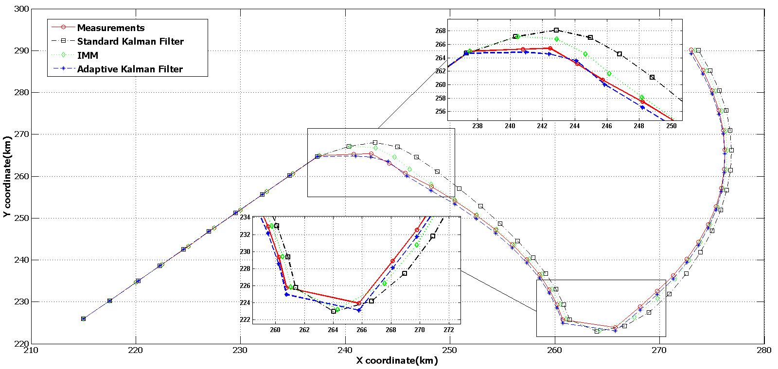
The three filters were run on simulated maneuvering trajectories and plotted against the measurements. The two figures below are the project's simulation outputs; what they do and do not show is set out beside them.

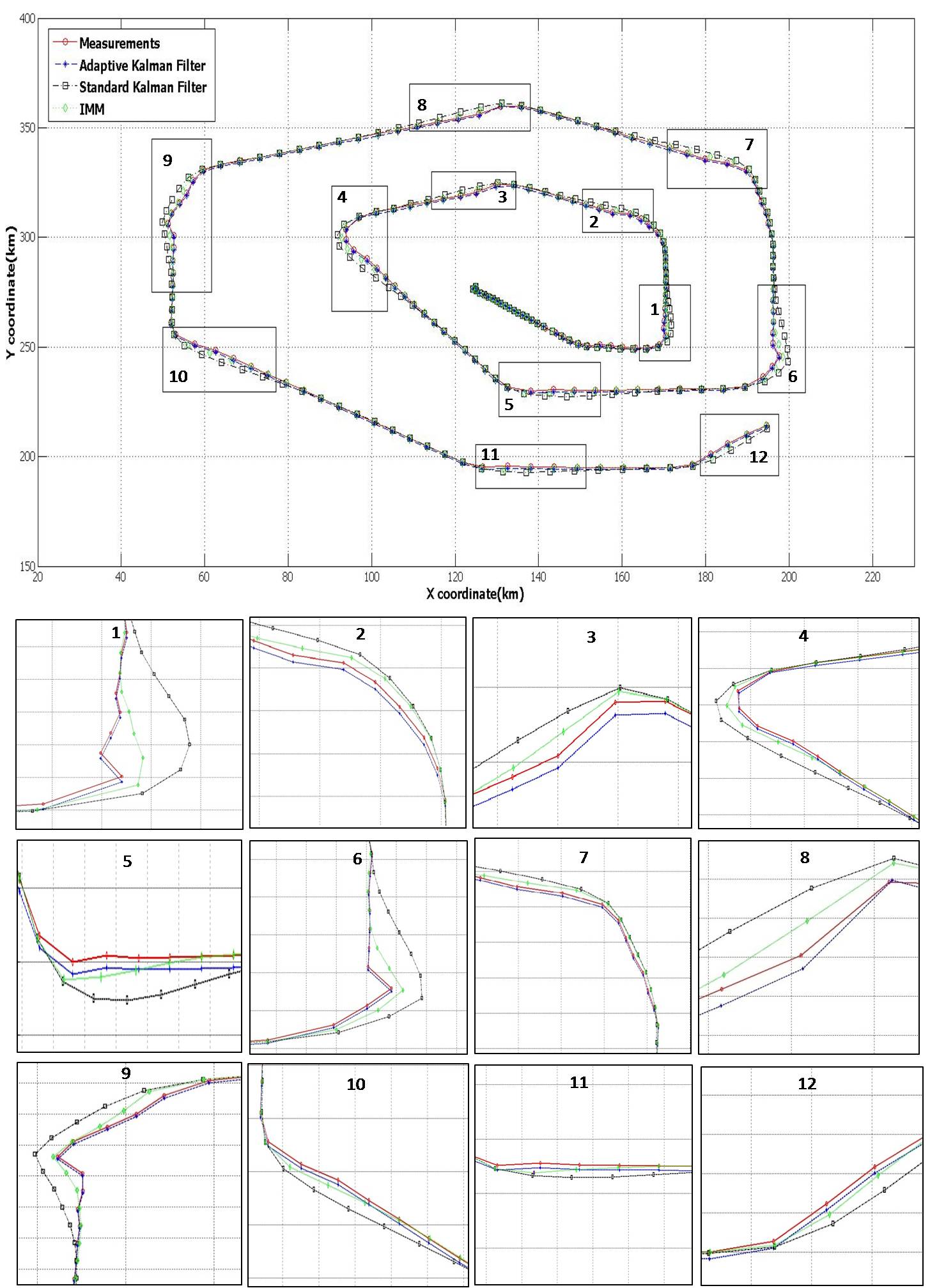
Scenario 1 simulation: X and Y coordinates in kilometres, with measurements in red circles, standard Kalman filter in black squares, IMM in green diamonds and adaptive Kalman filter in blue stars. Insets zoom into two turn regions. — Simulation result Scenario 1: a straight leg followed by a sequence of turns, with two turn regions enlarged.

Scenario 2 simulation: a long trajectory with many turns, X from 20 to 220 km and Y from 150 to 400 km, with twelve numbered boxes marking maneuver regions. Below the main plot, twelve enlarged panels show measurements, adaptive Kalman filter, standard Kalman filter and IMM in each region. — Simulation result Scenario 2: twelve maneuver regions, each enlarged below the main plot.

What the plots show

Straight segments: all three estimates overlap the measurements.
Turns: the standard Kalman filter estimate visibly swings wide and lags the measurement trace, most clearly in scenario 2 regions 1, 6 and 9.
IMM and adaptive KF: both stay closer to the measurement trace through the turns; in many enlarged regions the adaptive estimate is the closest of the three.
Not uniform: in some regions (e.g. 3 and 5) the adaptive estimate sits visibly offset from the measurements, so the advantage is not the same at every maneuver.

How to read them. The plots compare each estimate with the noisy measurements, not with a true trajectory, and come from individual runs. Following the measurements closely is not the same as lower estimation error. No RMSE, Monte Carlo statistics or timing results accompany them, and the noise levels, scan interval and filter tuning are not documented in the files.

Test scenarios for a full evaluation

Approximately constant-velocity motion
Abrupt heading change
Sudden acceleration or deceleration
Repeated maneuvers
Noisy position measurements, with and without clutter

Metrics to measure

Position error and RMSE against the true trajectory
Track continuity through each maneuver
Measurement-association behavior
Maneuver-response delay
Processing time per scan and computational cost

These are evaluation criteria for the three approaches under identical conditions, not reported results.

“Zero processing latency”Stated in earlier project notes. Every filter takes some execution time, so this needs measured per-scan timing before it is presented as a result; it is not claimed on this page.

Lower complexity than IMM / EKFPlausible from the structure (one filter instead of several), but it should be confirmed by operation counts or timing on the same hardware.

Multi-target performanceThe design targets multi-target tracking, but the available plots show single-target scenarios; association behavior with several targets and clutter remains to be demonstrated.

Key takeaways

Engineering Contributions

The project explores how a targeted change to the prediction and association stages can help a Kalman-based tracker respond to changing target motion, instead of replacing the filter with a heavier multiple-model structure.

Kalman filtering and recursive state estimation
Target-motion modeling
Maneuver detection and model mismatch
Adaptive predicted-position correction
Innovation and residual analysis
Validation gating and measurement association
Multi-target tracking concepts
Computational-efficiency considerations
Simulation-based comparison with standard KF and IMM

Illustration titled Practical Applications: air defense systems, military surveillance in C4I systems, UAV and drone tracking for counter-UAV and unmanned traffic management, and aerospace and autonomous systems for navigation and collision avoidance. — Project illustration Application areas where maneuvering targets are common.

Contact & Collaboration

Working on Target Tracking or State Estimation?

I welcome discussions about Kalman filtering, maneuvering-target tracking, data association and tracking R&D collaboration.

Send an Email LinkedIn All Projects

Adaptive Kalman Filtering for Maneuvering Targets

Rapid Evasive Maneuvers

Constant-velocity assumption

Abrupt heading change

Sudden acceleration or deceleration

Unexpected direction change

Model mismatch → growing residuals

Possible divergence

Standard Kalman Filter Fundamentals

PREDICT Project the state ahead

UPDATE Correct with the measurement

Notation

Interacting Multiple Model (IMM) Algorithm

IMM structure, one scan

Maneuver Detection

Normalized innovation squared

Residual evidence over successive scans

Proposed Adaptive Kalman Tracking Algorithm

Why shift the prediction?

Conceptual processing sequence

The position shift

Two different levers

Validation gate: standard vs. shifted

Recentering the gate after a maneuver

Algorithm Workflow

Comparison of Tracking Approaches

Simulation and Performance Evaluation

What the plots show

Test scenarios for a full evaluation

Metrics to measure

Engineering Contributions

Working on Target Tracking or State Estimation?