PROJECT 05 · ADAPTIVE TRACKING FILTERS

Adaptive Alpha–Beta Tracking Enhancement

AI-Based Adaptive Gains for Responsive, Low-Complexity Tracking

The alpha–beta tracker is popular because it is simple, fast and cheap to run. Its weakness is that its two gains, α and β, are fixed: values tuned for steady flight can make the track lag when the target speeds up, slows down or turns.

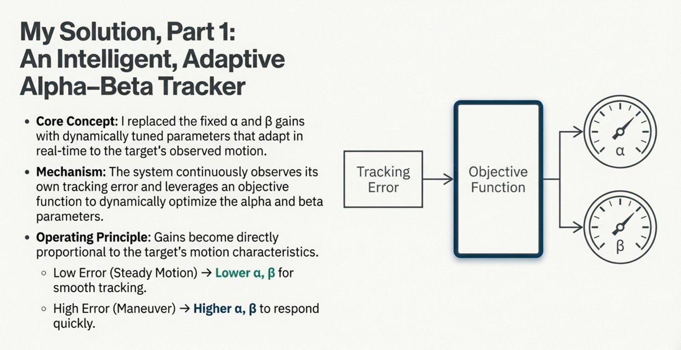
This project makes those gains adaptive. The tracker observes its own tracking deviations, evaluates them with an objective function and selects α and β to suit the target's current motion, while keeping the light recursive structure that makes alpha–beta tracking attractive for real-time systems.

Explore the Approach Compare with Kalman

Back to all projects

Project slide titled An Intelligent, Adaptive Alpha-Beta Tracker: tracking error feeds an objective function, which sets two dials labelled alpha and beta. Notes say the fixed gains are replaced by dynamically tuned parameters, lower gains are used for low error in steady motion and higher gains for high error during maneuvers. — Project illustration Core idea: tracking error → objective function → adapted α and β.

Baseline: Fixed-gain alpha–beta tracker (constant-velocity prediction)
Enhancement: α and β adapted from observed tracking deviations
Selection basis: An objective function that scores tracking performance
Design goal: Better response to changing motion at alpha–beta cost

The tracking problem

When Fixed Gains Meet Changing Motion

An alpha–beta tracker predicts each new position by assuming the target keeps its current velocity, then corrects that prediction with the measurement. For approximately constant-velocity motion, a well-chosen pair of gains gives a smooth, accurate track.

When the target accelerates, decelerates or changes direction, each prediction lands a little further from the measurement. With gains chosen for steady motion, the correction is too weak to catch up quickly: the estimate lags, and position and velocity errors grow until the filter settles on the new motion.

The choice of α and β sets the balance. Higher gains follow changes faster but pass more measurement noise into the track; lower gains smooth the noise but respond more slowly. One fixed pair cannot be ideal for every motion condition.

Fixed vs. adaptive gains through a turn

Conceptual, not simulation data

Drawn to explain the behavior, not computed from project data: with fixed gains the estimate overshoots the turn; adapted gains let it follow sooner.

Constant-velocity motion
The prediction model matches the target; well-tuned fixed gains track it accurately.
Sudden acceleration or deceleration
Predicted positions fall short of or overshoot the measurements.
Abrupt change in direction
The prediction continues along the old heading while the target turns.
Delayed response
Gains set for steady motion correct only part of the growing residual each update.
Growing estimation errors
Position and velocity errors build up until the filter settles on the new motion.
Responsiveness vs. noise
Raising the gains reduces lag but lets more measurement noise into the track.

Baseline algorithm

Standard Alpha–Beta Filter Fundamentals

Four steps per measurement, written here for one coordinate. A two-dimensional tracker applies the same structure to each position–velocity pair, e.g. x with its velocity and y with its velocity.

Step 1 · Predict position

${\hat{x}}_{k | k - 1} = {\hat{x}}_{k - 1 | k - 1} + {\hat{v}}_{k - 1 | k - 1} Δ t$

Extrapolates the last estimate at constant velocity over one interval.
Step 2 · Measurement residual

$r_{k} = z_{k} - {\hat{x}}_{k | k - 1}$

The deviation between the new measurement and the prediction.
Step 3 · Correct position

${\hat{x}}_{k | k} = {\hat{x}}_{k | k - 1} + α r_{k}$

Moves the prediction a fraction α of the way towards the measurement.
Step 4 · Correct velocity

${\hat{v}}_{k | k} = {\hat{v}}_{k - 1 | k - 1} + \frac{β}{Δ t} r_{k}$

Uses the same residual, scaled by β/Δt, to adjust the velocity estimate.

What the two gains do

Alpha: position correction
How strongly the predicted position is pulled towards the new measurement. α near 1 trusts the measurement; α near 0 trusts the prediction.
Beta: velocity correction
How strongly the residual changes the velocity estimate, and so how fast the tracker learns a new speed or direction.

A fixed pair can suit one motion condition well and another poorly. The best values also depend on the measurement interval $Δ t$ , the measurement noise and what the design is trying to minimise, so there is no single rule linking the gains directly to target speed.

Notation

$z_{k}$: Measured target position at time k.
${\hat{x}}_{k | k - 1}$: Predicted target position.
${\hat{x}}_{k | k}$: Corrected target position.
${\hat{v}}_{k - 1 | k - 1}$: Previous corrected velocity estimate.
${\hat{v}}_{k | k}$: Updated velocity estimate.
$r_{k}$: Measurement residual (deviation).
$α$: Position-correction gain.
$β$: Velocity-correction gain.
$Δ t$: Time between measurements.

Why adapt

Limitations of the Fixed-Gain Tracker

Fixed α and β cannot adjust themselves to every motion condition.
Low gains can cause excessive lag when the motion changes.
High gains make the estimate more sensitive to noisy measurements.
Poor tuning degrades performance in either direction.
The constant-velocity prediction does not explicitly model acceleration or turns.

None of this means an alpha–beta tracker fails during every maneuver. How well it copes depends on the gains, the measurement interval, the measurement quality and how sharply the target moves.

The responsiveness–noise trade-off

Illustrative, synthetic data

A standard alpha–beta filter run twice on the same synthetic, noisy measurements, once with low gains and once with high gains. Not project results.

The developed approach

Proposed Adaptive Alpha–Beta Enhancement

Instead of keeping α and β constant, the tracker adapts them using an AI-based parameter-adjustment concept: it learns from the deviations it observes under different target behaviors and picks gains that score best against an objective function.

Stage 1
Observe tracking behavior
Compare each prediction with the incoming observation and record the tracking deviation.
Stage 2
Relate deviations to motion
Consider the stored deviations under steady motion, acceleration or deceleration, and moderate maneuvering.
Stage 3
Score with an objective function
Evaluate tracking performance in a form that can be compared between candidate gains.
Stage 4
Select α and β
Choose the gains best suited to the observed condition and the target's motion characteristics.
Stage 5
Update the track
Apply the selected gains in the alpha–beta position and velocity corrections.
Stage 6
Keep monitoring
Continue observing residuals so the gains can respond to the next change in motion.

Adaptive gains, in general form

Illustrative formulation

The gains become functions of the information $φ_{k}$ available to the adaptation mechanism, such as recent tracking deviations or motion characteristics:

α_{k} = f_{α} (φ_{k})

β_{k} = f_{β} (φ_{k})

The corrections keep their standard form, using the selected gains:

{\hat{x}}_{k | k} = {\hat{x}}_{k | k - 1} + α_{k} r_{k}

{\hat{v}}_{k | k} = {\hat{v}}_{k - 1 | k - 1} + \frac{β_{k}}{Δ t} r_{k}

These expressions describe the structure only; the actual mapping from $φ_{k}$ to $α_{k}$ and $β_{k}$ is not given in the project files.

Documented direction of adaptation

Low deviation · steady motionLower α and β for a smooth track that is less affected by measurement noise.

High deviation · maneuverHigher α and β so the track responds quickly to the change in motion.

From the project's design summary. The exact gain values, limits and switching rules are not documented.

Intended engineering benefits

Better responsiveness to moderate changes in target motion
Less lag than a fixed pair of unsuitable gains
A flexible gain-adjustment mechanism
The simple recursive alpha–beta structure is retained
Potentially lower computation than more complex filters

Design aims; they have not yet been quantified with measured results.

About “AI-based”. The project describes an AI-based, objective-function-driven way of adapting the gains. The available files do not specify a neural network, training dataset, classifier or optimization algorithm, so none is claimed here.

How gains are chosen

Objective Function and Adaptive Gain Selection

An objective function turns “how well is the tracker doing?” into a number, so candidate gains can be compared and the best pair selected.

An error-based objective

Illustrative example

J (α, β) = \sum_{k = 1}^{N} w_{k} e_{k}^{2}

$J$: Objective function to be minimised.
$e_{k}$: Defined tracking error for sample k.
$w_{k}$: Optional weighting factor.
$N$: Number of samples in the evaluation interval.

The selection goal is the gain pair that minimises $J$ over the permitted range:

(α^{*}, β^{*}) = \underset{α, β}{\arg \min} J (α, β)

This is a typical form, not necessarily the implemented one. A design could add terms for velocity error, smoothness, responsiveness or gain stability; the gain limits and the search or optimization procedure must be defined by the implementation, and are not documented in the project files.

Why the best gains depend on motion

Illustrative

Curve shapes are invented for explanation. They show the documented direction of adaptation: larger deviations favour larger gains.

Tracking accuracy

The selected gains should reduce the chosen tracking error for the current motion condition.

Stability and noise sensitivity

Reacting aggressively to every residual can make the track jittery or unstable; one noisy measurement should not be mistaken for a maneuver.

One measurement, end to end

Adaptive Tracking Workflow

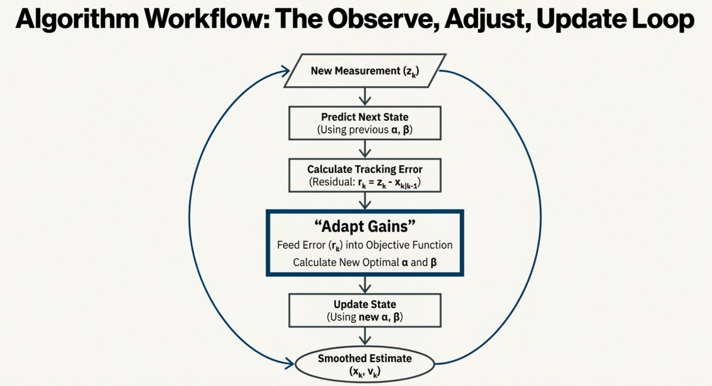
The standard alpha–beta cycle with an evaluation step that decides whether the gains should change before the correction is applied.

Start

Initialize target state and tracker parameters

Receive measurement

Predict position

Calculate residual

Record and evaluate tracking deviation

Evidence of changing motion?

Treat as ordinary measurement deviation; keep current α, β

YES

Evaluate motion condition

Determine suitable α and β via the objective function

Correct position

Correct velocity

Store updated track state

Process next measurement

Returns to “Receive measurement”. A single large residual is not, by itself, proof of a maneuver.

Project slide titled Algorithm Workflow, The Observe, Adjust, Update Loop: new measurement, predict next state, calculate tracking error as the residual, adapt gains by feeding the error into the objective function to calculate new alpha and beta, update state with the new gains, and output the smoothed estimate, looping back to the next measurement. — Project illustration The project's observe → adjust → update loop, summarised in the flowchart beside it.

Choosing a tracker

Alpha–Beta vs. Adaptive Alpha–Beta vs. Kalman Filter

No method is best everywhere. The right choice depends on the target dynamics, measurement quality, accuracy required and computing budget.

Qualitative comparison; no measured accuracy or timing figures are implied.
Criterion	Standard α–β	Adaptive α–β	Kalman Filter
Computational structure	Simple fixed-gain recursion.	Relatively simple, with adaptation overhead.	Depends on state dimension and model; covariance propagated every step.
Gain behavior	Fixed.	Adjusted by the adaptation mechanism.	Computed from the covariance and measurement models.
Constant-velocity tracking	Suitable when correctly tuned.	Suitable when correctly adapted.	Suitable with an appropriate model.
Changing motion	Can lag or accumulate errors.	Designed to improve responsiveness.	Depends on the selected motion model.
Noise handling	Controlled indirectly through the gains.	Depends on adaptation and tuning.	Explicitly represents process and measurement uncertainty.
Implementation complexity	Low.	Low to moderate, depending on the adaptation method.	Model-dependent.
Main trade-off	Simplicity versus adaptability.	Adaptability versus tuning and validation requirements.	Model sophistication versus computational cost.

In brief

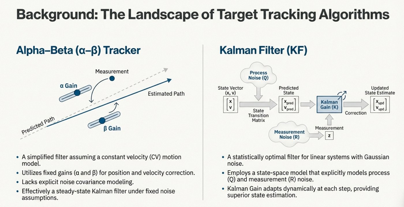
Standard α–β: simple recursion, low computation and easy implementation; fixed gains can lag or accumulate error when the motion no longer suits them.

Adaptive α–β: gains selected from stored tracking deviations through an objective-function-driven mechanism, aiming for better responsiveness in a lightweight structure. Its value depends on how well the adaptation is designed and validated.

Kalman filter: explicit state and covariance estimation with process- and measurement-noise models. Under its linear-Gaussian assumptions it gives the minimum-variance linear estimate, at the cost of more modeling and implementation effort in many applications. It also supports richer motion models.

Project slide titled The Landscape of Target Tracking Algorithms. Left: the alpha-beta tracker, with alpha and beta gain sliders pulling a predicted path towards a measurement; notes say it assumes constant velocity, uses fixed gains, lacks explicit noise covariance modeling and is effectively a steady-state Kalman filter. Right: a Kalman filter block diagram with process noise Q, measurement noise R, Kalman gain K and the predicted and updated state. — Project illustration Alpha–beta as a fixed-gain, steady-state special case; the Kalman filter recomputes its gain from explicit noise models.

Engineering perspective

Maneuvering-Target Tracking

Standard alpha–beta filter

Its basic constant-velocity prediction does not explicitly model arbitrary acceleration.
Behavior depends on gain tuning.
Can lag noticeably during evasive maneuvers when the gains do not suit the motion.
The adaptive enhancement targets exactly this gap, while keeping the same structure.

Kalman filter

Estimates state and error covariance recursively, and can be built on motion models suited to the expected maneuvers:

Constant acceleration (CA): adds acceleration to the state for speed changes.
Coordinated turn (CT): models turning at a constant rate.
Heading-augmented: carries heading in the state to represent direction changes.

No guaranteed winner. A well-chosen model helps a Kalman filter track the matching motion pattern, but a correctly designed Kalman filter is not certain to beat every alpha–beta implementation in every scenario. Model suitability, tuning, measurements and computational limits all decide the outcome.

Validation plan

Simulation and Performance Evaluation

How the adaptive tracker should be compared with a fixed-gain alpha–beta filter and a Kalman filter.

No simulation results are shown yet. The project files contain concept slides but no result plots or data, so this section sets out the method rather than reporting numbers.

Test scenarios

Constant-velocity motion
Acceleration
Deceleration
Moderate changes in heading
Noisy measurements
Different measurement sampling intervals

Metrics to measure

Position RMSE against the true trajectory
Velocity-estimation error
Tracking lag and response to changes in motion
Sensitivity to measurement noise
Processing time per update
Computational cost

All three trackers should run on identical simulated trajectories and noise, with Monte Carlo repetition, so differences come from the algorithms rather than from a single lucky run.

Performance “comparable to more complex filters”Stated in one project slide; it needs RMSE and lag comparisons against a Kalman filter before it can be presented as a result.

Low computational cost retainedPlausible from the structure, but the adaptation overhead should be measured as time or operations per update.

The AI-based adaptation itselfThe method (classifier, optimizer or learned mapping), its training data and gain limits need to be documented to support the description.

Where it could fit

Engineering Benefits and Applications

Potential application areas for lightweight adaptive tracking, each subject to its own validation. These are not claimed deployments.

Radar surveillance
Air Traffic Control (ATC)
Command and Control (C2 / C4I)
GPS-based vehicle tracking
Autonomous vehicles
Robotics and mobile platforms
Real-time systems with limited computing resources

The trade-off

Fixed-gain alpha–beta is cheap but inflexible. Adaptive alpha–beta seeks flexibility without losing the simple recursion. A Kalman filter offers a more explicit estimation framework whose performance depends on its model and noise assumptions.

Conclusion

Engineering Conclusion

The alpha–beta tracker is attractive when computational simplicity and fast execution are priorities. Its basic constant-velocity prediction and fixed gains do not stop it from responding to acceleration, but they can produce larger errors when target dynamics change. The proposed enhancement seeks to improve that behavior by using observed deviations and an objective-function-driven approach to adjust α and β dynamically, a practical direction for lightweight real-time tracking.

The Kalman filter provides a more general state-estimation framework and supports richer motion models, including constant-acceleration and coordinated-turn models. The right choice depends on the target dynamics, measurement quality, required accuracy, computational budget and, ultimately, validation results.

Contact & Collaboration

Building Real-Time Trackers?

I welcome discussions about alpha–beta and Kalman tracking, adaptive filtering, tracking-error analysis and tracking R&D collaboration.

Send an Email LinkedIn All Projects

Adaptive Alpha–Beta Tracking Enhancement

When Fixed Gains Meet Changing Motion

Fixed vs. adaptive gains through a turn

Constant-velocity motion

Sudden acceleration or deceleration

Abrupt change in direction

Delayed response

Growing estimation errors

Responsiveness vs. noise